Jwif: You're right, it doesn't work like [line~]. I think the idea Andy's trying to present it that with a lowpass filter you can create curved transitions instead of lines.

ymotion: The high frequency content can be a difficult concept to wrap one's head around at first. Basically, when you have a sudden jump between two samples (say from 0 to 1) you have what's called a discontinuity. Now, according to Fourier theory, signals can be defined as a sum of sinusoids at different frequencies. The only way to create a discontinuity is for there to be an infinite number of frequencies that happen to be perfectly in phase at that exact moment. So, every time you move the slider, [sig~] is making a sudden jump from the last value to the new one. The lowpass filter is getting rid of a lot of the high frequencies, which has the effect of smoothing it out.

I fairly recently was trying to make one of those smoothed-out sample-and-hold LFOs and discovered that [lop~] generates asymmetric curves: logarithmic going up and exponential going down. It definitely was not useful in that situation. I was looking more for an S-curve. Turns Bessel filters do this (they also slightly overshoot the target value and oscillate a little before settling--something to keep in mind). If you wanted to get a straight line between values, a moving average filter will do that. Basically what I'm saying here is, if you have a preferred curve in mind, try out different filters to find the closest one.

The attached patch should help to visualize the curves.

http://www.pdpatchrepo.info/hurleur/smoothsteps.mmb.pd

copy below dots in notepad etc...safe as ansi name.pd
........................................................................................................................
#N canvas 413 15 740 910 10;
#N canvas 559 52 558 609 fft 0;
#X obj 19 61 inlet~;
#X obj 195 217 inlet;
#X obj 29 92 rfft~;
#X obj 29 125 *~;
#X obj 60 125 *~;
#X obj 29 155 sqrt~;
#X obj 29 181 biquad~ 0 0 0 0 1;
#X text 93 93 Fourier series;
#X text 98 146 magnitude;
#X text 96 131 calculate;
#X text 21 3 This subpatch computes the spectrum of the incoming signal
with a (rectangular windowed) FFT. FFTs aren't properly introduced
until much later.;
#X text 83 61 signal to analyze;
#X text 193 164 delay two samples;
#X text 191 182 for better graphing;
#X obj 231 236 inlet;
#X text 284 234 toggle to graph repeatedly;
#X text 262 212 bang to graph once;
#X obj 19 295 tabwrite~ E09-signal;
#X obj 231 298 tabwrite~ E09-spectrum;
#X obj 29 205 /~ 4096;
#X msg 195 322 \; pd dsp 1;
#X obj 231 259 metro 70;
#X obj 332 109 block~ 4096 1;
#X obj 31 237 *~ 10;
#X connect 0 0 2 0;
#X connect 0 0 17 0;
#X connect 1 0 17 0;
#X connect 1 0 18 0;
#X connect 1 0 20 0;
#X connect 2 0 3 0;
#X connect 2 0 3 1;
#X connect 2 1 4 0;
#X connect 2 1 4 1;
#X connect 3 0 5 0;
#X connect 4 0 5 0;
#X connect 5 0 6 0;
#X connect 6 0 19 0;
#X connect 14 0 20 0;
#X connect 14 0 21 0;
#X connect 19 0 23 0;
#X connect 21 0 17 0;
#X connect 21 0 18 0;
#X connect 23 0 18 0;
#X restore 50 125 pd fft;
#X obj 109 68 bng 18 250 50 0 empty empty empty 0 -6 0 8 -262144 -1
-1;
#X obj 109 89 tgl 18 1 empty empty empty 0 -6 0 8 -262144 -1 -1 1 1
;
#N canvas 0 0 450 300 (subpatch) 0;
#X array E09-signal 882 float 0;
#X coords 0 1.02 881 -1.02 200 80 1;
#X restore 207 18 graph;
#N canvas 0 0 450 300 (subpatch) 0;
#X array E09-spectrum 259 float 0;
#X coords 0 0.51 258 -0.008 259 130 1;
#X restore 179 129 graph;
#X text 216 104 ---- 0.02 seconds ----;
#X text 271 147 SPECTRUM;
#X obj 24 512 gemwin;
#X obj 24 467 tgl 15 0 empty empty empty 17 7 0 10 -262144 -1 -1 1
1;
#X msg 50 469 create;
#X msg 53 489 destroy;
#X obj 191 288 gemhead;
#X obj 191 339 t a a a;
#X obj 180 368 GEMglEnd;
#X obj 236 367 GEMglBegin;
#X obj 362 350 GLdefine GL_LINES;
#X obj 362 320 loadbang;
#X obj 341 321 bng 15 250 50 0 empty empty empty 17 7 0 10 -262144
-1 -1;
#X obj 209 508 gemlist;
#X obj 209 429 f 256;
#X obj 209 448 until;
#X obj 208 472 t b b;
#X obj 293 470 + 1;
#X obj 210 396 t b b a;
#X obj 276 446 f 0;
#X obj 262 469 f;
#X obj 210 547 GEMglVertex2f;
#X obj 210 603 GEMglVertex2f;
#X obj 295 560 * -1;
#X obj 260 526 - 4;
#X obj 191 312 translateXYZ;
#X floatatom 242 288 5 0 0 0 - - -;
#X obj 295 520 tabread E09-spectrum;
#X obj 260 506 / 32;
#X obj 52 12 adc~;
#X obj 51 39 hip~ 5;
#X obj 51 65 *~ 1;
#X floatatom 94 42 5 0 0 0 - - -;
#X obj 210 579 spigot;
#X obj 149 564 tgl 15 0 empty empty empty 17 7 0 10 -262144 -1 -1 0
1;
#X text 404 -74 i think its a bouchard patch;
#X text 66 578 just for the symetry;
#X connect 1 0 0 1;
#X connect 2 0 0 2;
#X connect 8 0 7 0;
#X connect 9 0 7 0;
#X connect 10 0 7 0;
#X connect 11 0 30 0;
#X connect 12 0 13 0;
#X connect 12 1 23 0;
#X connect 12 2 14 0;
#X connect 15 0 14 1;
#X connect 16 0 15 0;
#X connect 17 0 15 0;
#X connect 18 0 26 0;
#X connect 19 0 20 0;
#X connect 20 0 21 0;
#X connect 21 0 18 0;
#X connect 21 1 25 0;
#X connect 22 0 25 1;
#X connect 23 0 19 0;
#X connect 23 1 24 0;
#X connect 23 2 18 1;
#X connect 24 0 25 1;
#X connect 25 0 22 0;
#X connect 25 0 33 0;
#X connect 25 0 32 0;
#X connect 26 0 38 0;
#X connect 28 0 27 2;
#X connect 29 0 26 1;
#X connect 29 0 27 1;
#X connect 30 0 12 0;
#X connect 31 0 30 1;
#X connect 32 0 26 2;
#X connect 32 0 28 0;
#X connect 33 0 29 0;
#X connect 34 0 35 0;
#X connect 35 0 36 0;
#X connect 36 0 0 0;
#X connect 37 0 36 1;
#X connect 38 0 27 0;
#X connect 39 0 38 1;

Hi.

Does anyone have experience working with bezier curves? I'm having a little trouble getting my head around the formulas.

What I'd like to do is to define half a saturation curve with the visual output of an array in bezier curve mode.

So I have an array with five points in it. The first point is locked to 0,0, the last point locked to 1,1. the three intermediate points are editable by a selector and a slider.

Visually in the graph, the result is a nice-looking bezier curve. Of course, there's only five points here. So I need a way to upsample those five points in a bezier fashion. The result would be an array with many points in it that match the curve of the original visual bezier.

I'll attach a sloppy patch to illustrate, if anyone can steer me in the right direction that would be swell, but no hard feelings if you're not feeling it.

thanks kindly folks.

http://www.pdpatchrepo.info/hurleur/lxi_bezier.pd

A very interesting approach to give sequencers a feeling is called "groove mapping". Sofwares like live or acid implement it.

Basically, the idea is to separate the groove/feeling from the score, so that you can apply the groove to any score. The main parameters are velocity, duration and timeshift for every note position.

It enables you to write new scores that automatically groove or swing, without editing individual notes. I used this principle for the swing in the patch posted there: http://puredata.hurleur.com/sujet-4544-drums4dummies, though it is a standalone player from which all barely usable editing stuff was removed.

My implementation of groove mapping is very messy as I started to learn pd for this purpose, but I'd be happy to share it with anyone interested.

@Maelstorm said:

If you're on OSX, jack can be used as an insert plug-in so you can avoid the separate tracks, but you still get the latency.

which you can, depending on your host, eliminate by setting the track delay for the track with the plugin. So if the buffer is 512 sample/11.82 ms then set the delay to that and it should be spot on.

I've had the whole Jack graph latency explained to me numerous times by Stephane Letz and it still doesn't go in.....Heres what he told me...

> > Its the Pd > JAck > Ableton latency. (Ableton has otoh 3 different
> > ways of manually setting latency compensation - I'm just not very
> > clear on where to start with regards to input from JAck)
> >>>>
>
> This is NO latency introduced in a Pd > JAck > Ableton kind of
> chain; the JACK server activate each client in turn (that is Pd *then*
> Ableton in this case) in the *same* given audio cycle.
>
> Remember : the JACK server is able to "sort" (in some way) the graph
> of all connected clients to activate each client audio callback at the
> right place during the audio cycle. For example:
>
> 1) in a sequential kind of graph like IN ==> A ==> B ==> C ==> OUT,
> JACK server will activate A (which would typically consume new audio
> buffers available in machine audio IN drivers) then activate B (which
> would typically consume "output" just produced by A) , then activate
> C , then produce the machine OUT audio buffers.
>
> 2) in a graph will parallel sub-graph like : IN ==> A ==> B ==> C
> ==> OUT and IN ==> D ==> B ==> C ==> OUT (that is both A and D are
> connected to input and send to , then JACK server is able to
> activate A and D at the same time (since the both only depends of IN)
> and a multi-core machine will typically run A and D at the same time
> on 2 different cores. Then when A *and* D are finished, B can be
> activated... and so on.
>
> The input/output latency of a usual CoreAudio application running
> is: driver input latency + driver input latency offset + 2
> application buffer-size + driver output latency + driver output
> latency offset.
>

this next part is the important bit i think...

> For a graph of JACK clients: driver input latency + driver input
> latency offset + 2 JACK Server buffer-size + ( one extra buffer-
> size ) + driver output latency + driver output latency offset.
>
> (Note : there is an additional one extra buffer-size latency on OSX,
> since the JACK server is running in the so called "asynchronous" mode
> [there is also a "synchronous" mode without this one extra buffer-size
> available, but it is less reliable on OSX and we choose to use the
> "asynchronous" mode by default.])
>
> Stephane
>

what's your soundcard's sampling rate? tabwrite~ will only display the graph once all the data has been read into the graph.

your graph is 6000 samples long, and your metro is 200ms. so at 44100hz, 200ms = 8820 samples, so because the graph is full, it is displayed.

but if you have a lower sampling rate, say 22050hz, then 200ms will only graph 4410 samples. because this is less than the size of the graph, the tabwrite~ is retriggered before the graph is full, and thus will not display the output. a smaller graph should help, hopefully.

Hopefully this graph will help explain it Shankar,

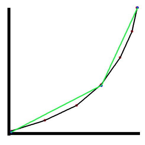
Firstly, in the case of this graph, lets say that we know that our data will lead to a perfect curve.

The red nodes, would be the scaled down points you would get from something like scaling 127 into 1.
The black line follows the path of that data. You can see because of limited reference points, we dont end up with a smooth curve, we are skipping whats inbetween and connecting what we do know.

The blue nodes, would be something scaled up, like scaling 127 into 400.
Now, our reference points are further apart, so we have less data to make our curve with.
The green line follows this curve, which isn't too much of a curve because we have even less data.

Basically, what im saying is, that the reason scaling 127 into 1 works, is because you have a higher resolution of data, more points to reference, so you get a smoother transition.

I guess a better example to use in this case would be steps though.

hi, i'm new to puredata and i have a problem about graphs,
for example, i create a graph and i want to put some bangs, some toggles.. inside,
i edit the graph with right click->open, when i close it and look at the graph at parent patch all GUI objects are messed up - misplaced..
is there any way that i can decorate these graph objects properly?

for example,
i have a graph width 200- height 150
i want my toggles to be at a specific position (x,y) like (10,25) (30,25) (50 25)...
is that possible?
thanx

With tabread4~ what's happening is that a sliding window of 4 samples is moving forwards and the instantaneous output is a function of those four values. It's done to smooth the curve of the data when the sampling points might not be accurate (because of say quantisation errors), and also to provide access to values in between the real stored values. This happens when you want to read the sample of looping oscillator back at a frequency that isn't an integer factor of the original sample rate - common for most oscillators. Imagine you had a table of just 2 samples. 2 point linear interpolation would say - if value 0 is 10 and value 1 is 20 then the value that *would* be at index 0.5 (if it existed) is 15 (the simple average) That's interpolation. Theres many takes on it, which fall under the numerical methods field of "curve fitting" you might find better examples searching on that term. Polynomials are cool because they are infinitely differentiable, you can pick any in between value and it will fit smoothly into the curve with the others and won't suddenly freak out to infinity or zero.

Basically -

Linear, we just take two points and assume a line runs between them to find an inbetween value.

Polynomial (2nd order) We use an equivillence like Legrange (turns a sequence to sum of products) which are coefficients of a polynomial (eg S = 1x + 3y + 16z^2)
That gives us a curve that can fit to three points.

There's cubic (spline) and other interpolation functions you can use. Basically the higher the order of powers the more smoothness and accuracy you will get, but you will need to process more samples for each table read .

http://www.efunda.com/math/num_interpolation/num_interpolation.cfm